Sparse recovery
The aim is to recover a sparse nonnegative signal \(x_0 \in \mathbb{R}^n\) from a measurement vector \(y = A x_0\), where \(A \in \mathbb{R}^{m \times n}\) (with \(m < n\)) is a known sensing matrix. A common heuristic based on convex optimization is to minimize the \(\ell_1\) norm of \(x\) (which reduces here to the sum of entries of \(x\)) subject to \(y = Ax_0\) (and here, \(x \geq 0\)).
It has been proposed to minimize the sum of the square roots of the entries of \(x\), which since \(x \geq 0\) is the same as minimizing the square root of the \(\ell_{1/2}\) ‘norm’ (which is not convex, and therefore not a norm), to obtain better recovery.
The optimization problem is
where \(x\) is the variable. (The constraint \(x \geq 0\) is implicit, since this is the objective domain.) This is a nonconvex problem, directly in DCCP form.
[1]:
import cvxpy as cp
import matplotlib.pyplot as plt
import numpy as np

from dccp import is_dccp

rng = np.random.default_rng()

n = 100
m = [50, 56, 62, 68, 74, 80]
k = [30, 34, 38, 42, 46, 50]
T = 3

proba = np.zeros((len(m), len(k)))
proba_l1 = np.zeros((len(m), len(k)))

for time in range(T):
    for kk in k:
        x0 = np.zeros((n, 1))
        ind = rng.permutation(n)
        ind = ind[0:kk]
        x0[ind] = rng.standard_normal((kk, 1)) * 10
        x0 = np.abs(x0)

        for mm in m:
            A = rng.standard_normal((mm, n))
            y = np.dot(A, x0)

            # sqrt of 0.5-norm minimization
            x_pos = cp.Variable(shape=((n, 1)), nonneg=True)
            cost = cp.reshape(cp.sum(cp.sqrt(x_pos), axis=0), (1, 1), order="F")
            prob = cp.Problem(cp.Minimize(cost), [A @ x_pos == y])

            # initialize variable value before solving
            x_pos.value = np.ones((n, 1))
            assert is_dccp(prob)

            # try different solvers in case one fails
            result = None
            try:
                result = prob.solve(method="dccp", solver=cp.ECOS)
            except Exception:
                pass

            if result is None:
                x_pos.value = None

            norm_diff = cp.pnorm(x_pos - x0, 2).value
            norm_x0 = cp.pnorm(x0, 2).value
            if (
                x_pos.value is not None
                and norm_diff is not None
                and norm_x0 is not None
                and norm_diff / norm_x0 <= 1e-2
            ):
                indm = m.index(mm)
                indk = k.index(kk)
                proba[indm, indk] += 1 / float(T)

            # l1 minimization
            xl1 = cp.Variable((n, 1))
            cost_l1 = cp.pnorm(xl1, 1)
            obj = cp.Minimize(cost_l1)
            constr = [A @ xl1 == y]
            prob_l1 = cp.Problem(obj, constr)
            result_l1 = prob_l1.solve()

            norm_diff = cp.pnorm(xl1 - x0, 2).value
            norm_x0 = cp.pnorm(x0, 2).value
            if norm_diff is not None and norm_x0 is not None and norm_diff / norm_x0 <= 1e-2:
                indm = m.index(mm)
                indk = k.index(kk)
                proba_l1[indm, indk] += 1 / float(T)

# validate outputs
assert np.all(proba >= 0) and np.all(proba <= 1)
assert np.all(proba_l1 >= 0) and np.all(proba_l1 <= 1)
/home/langestefan/dev/cvx/dccp/.venv/lib64/python3.13/site-packages/cvxpy/problems/problem.py:1539: UserWarning: Solution may be inaccurate. Try another solver, adjusting the solver settings, or solve with verbose=True for more information.
  warnings.warn(
Experimental result
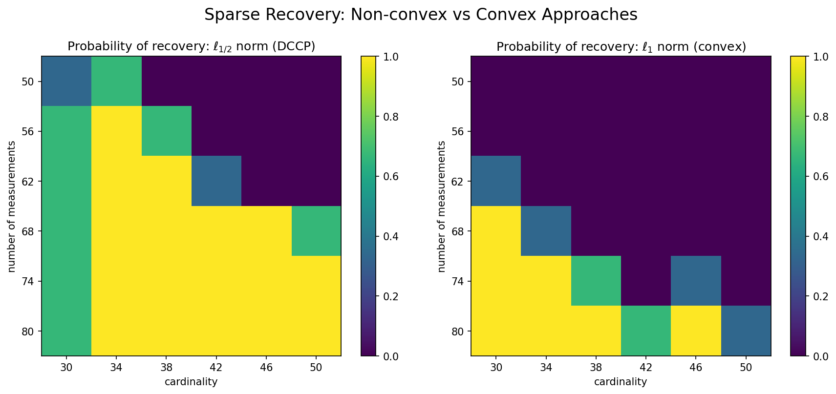
In a numerical simulation, we take \(n=100\), \(A_{ij} \sim \mathcal{N}(0,1)\), the positions of the nonzero entries in \(x_0\) are from uniform distribution, and the nonzero values are the absolute values of \(\mathcal{N}(0,100)\) random variables.
To count the probability of recovery, 100 independent instances are tested, and a recovery is successful if the relative error
is less than 0.01.
In each instance, the cardinality takes 6 values from 30 to 50, according to which \(x_0\) is generated, and \(A\) is generated for each \(m\) taking one of the 6 values from 50 to 80. The results in the figure below verify that nonconvex recovery is more effective than convex recovery.
[2]:
fig = plt.figure(figsize=[12, 5], dpi=150)
ax = plt.subplot(1, 2, 1)

plt.xticks(range(len(k)), k)
plt.xlabel("cardinality")
plt.yticks(range(len(m)), m)
plt.ylabel("number of measurements")

a = ax.imshow(proba, interpolation="none")
fig.colorbar(a)
ax.set_title(r"Probability of recovery: $\ell_{1/2}$ norm (DCCP)")
ax = plt.subplot(1, 2, 2)
b = ax.imshow(proba_l1, interpolation="none")
fig.colorbar(b)
plt.xticks(range(len(k)), k)
plt.xlabel("cardinality")
plt.yticks(range(len(m)), m)
plt.ylabel("number of measurements")
ax.set_title(r"Probability of recovery: $\ell_1$ norm (convex)")

# Add overall title
fig.suptitle("Sparse Recovery: Non-convex vs Convex Approaches", fontsize=16, y=1.02)
plt.tight_layout()