Gaussian covariance matrix estimation
Suppose \(y_i \in \mathbb{R}^n\) for \(i = 1, \ldots, N\) are points drawn i.i.d.from \(\mathcal{N}(0,\Sigma)\). Our goal is to estimate the parameter \(\Sigma\) given these samples.
The maximum likelihood problem of estimating \(\Sigma\) is convex in the inverse of \(\Sigma\), but not \(\Sigma\).
If there are no other constraints on \(\Sigma\), the maximum likelihood estimate is
the empirical covariance matrix.
[1]:
"""DCCP package."""

import matplotlib.pyplot as plt
import numpy as np
import cvxpy as cp
from dccp import is_dccp

rng = np.random.default_rng(0)
n = 20
N = 30
mean = [0, 0, 0, 0, 0, 0, 0, 0, 0, 0, 0, 0, 0, 0, 0, 0, 0, 0, 0, 0]
cov = np.eye(n)

for i in range(0, n - 3):
    cov[i, i + 3] = -0.2
    cov[i + 3, i] = -0.2
for i in range(0, n - 6):
    cov[i, i + 6] = 0.6
    cov[i + 6, i] = 0.6
pos = cov > 0
neg = cov < 0
zero = cov == 0

y = np.zeros((n, N))
Sigma = cp.Variable((n, n))

t = cp.Variable(1)
cost = cp.log_det(Sigma) + t
t.value = [1]
Sigma.value = np.eye(n)

emp = np.zeros((n, n))
for k in range(N):
    y[:, k] = rng.multivariate_normal(mean, cov)
    emp = emp + np.outer(y[:, k], y[:, k]) / N
temp = cp.sum([cp.matrix_frac(y[:, i], Sigma) / N for i in range(N)])
trace_val = temp
constr = [
    trace_val <= t,
    cp.multiply(pos, Sigma) >= 0,
    cp.multiply(neg, Sigma) <= 0,
    cp.multiply(zero, Sigma) == 0,
]
prob = cp.Problem(cp.Minimize(cost), constr)
assert is_dccp(prob)
result = prob.solve(method="dccp", max_iter=10, solver="SCS",
    max_slack=1e-3, eps=1e-3, seed=0
)
assert result is not None
assert Sigma.value is not None
Numerical example
We consider here the case where the sign of the off-diagonal entries in \(\Sigma\) is known; that is, we know which entries of \(\Sigma\) are negative, which are zero, and which are positive. (So we know which components of \(y\) are uncorrelated, and which are negatively and positively correlated.)
The maximum likelihood problem is then
where \(\Sigma\) is the variable, and the index sets \(\Omega_+\), \(\Omega_-\), and \(\Omega_0\) are given. The objective is a difference of convex functions, so we transform the problem into the following DCCP problem with additional variable \(t\),
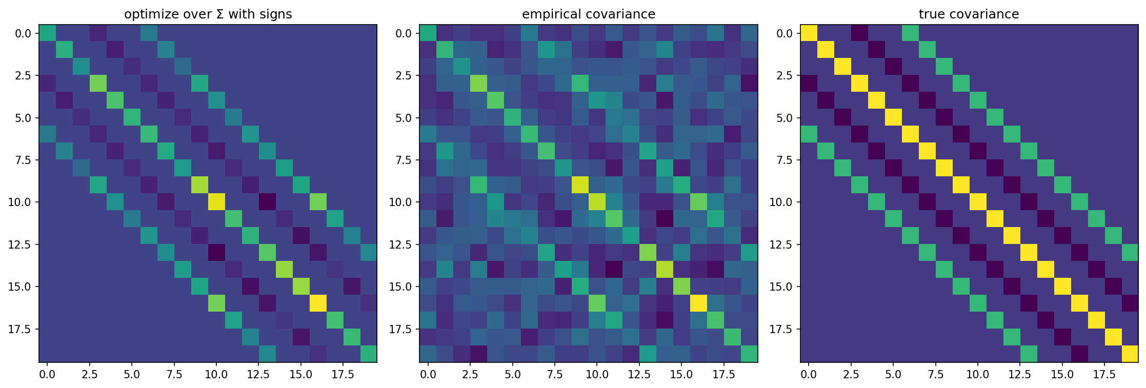
An example with \(n=20\) and \(N=30\) is shown below.
Not surprisingly, knowledge of the signs of the entries of \(\Sigma\) allows us to obtain a much better estimate of the true covariance matrix.
[2]:
plt.figure(figsize=(15, 5), dpi=150)
plt.subplot(131)
plt.imshow(Sigma.value, interpolation="none")
plt.title("optimize over $\Sigma$ with signs")
plt.subplot(132)
plt.imshow(emp, interpolation="none")
plt.title("empirical covariance")
plt.subplot(133)
plt.imshow(cov, interpolation="none")
plt.title("true covariance")
plt.tight_layout()