Total variation in-painting#
Grayscale Images#
A grayscale image is represented as an \(m \times n\) matrix of intensities \(U^\mathrm{orig}\) (typically between the values \(0\) and \(255\)). We are given the values \(U^\mathrm{orig}_{ij}\), for \((i,j) \in \mathcal K\), where \(\mathcal K \subset \{1,\ldots, m\} \times \{1, \ldots, n\}\) is the set of indices corresponding to known pixel values. Our job is to in-paint the image by guessing the missing pixel values, i.e., those with indices not in \(\mathcal K\). The reconstructed image will be represented by \(U \in {\bf R}^{m \times n}\), where \(U\) matches the known pixels, i.e., \(U_{ij} = U^\mathrm{orig}_{ij}\) for \((i,j) \in \mathcal K\).
The reconstruction \(U\) is found by minimizing the total variation of \(U\), subject to matching the known pixel values. We will use the \(\ell_2\) total variation, defined as $\(\mathop{\bf tv}(U) = \sum_{i=1}^{m-1} \sum_{j=1}^{n-1} \left\| \left[ \begin{array}{c} U_{i+1,j}-U_{ij}\\ U_{i,j+1}-U_{ij} \end{array} \right] \right\|_2.\)$ Note that the norm of the discretized gradient is not squared.
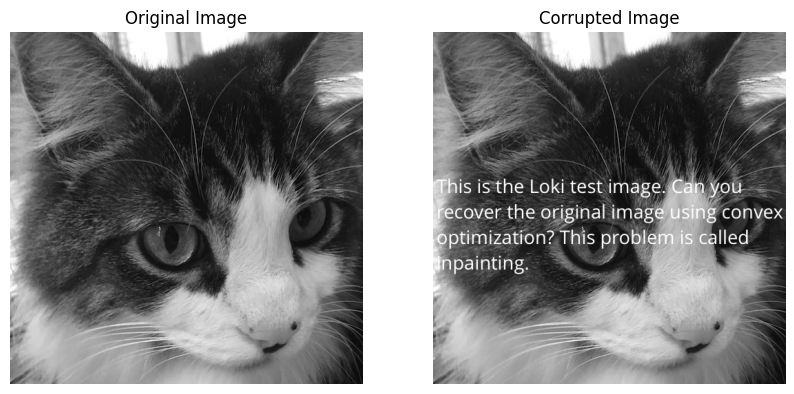
We load the original image and the corrupted image and construct the Known matrix. Both images are displayed below. The corrupted image has the missing pixels whited out.
import matplotlib.pyplot as plt
import numpy as np

# Load the images.
u_orig = plt.imread("data/loki512.png")
u_corr = plt.imread("data/loki512_corrupted.png")
rows, cols = u_orig.shape

# known is 1 if the pixel is known,
# 0 if the pixel was corrupted.
known = np.zeros((rows, cols))
for i in range(rows):
    for j in range(cols):
        if u_orig[i, j] == u_corr[i, j]:
            known[i, j] = 1

fig, ax = plt.subplots(1, 2, figsize=(10, 5))
ax[0].imshow(u_orig, cmap="gray")
ax[0].set_title("Original Image")
ax[0].axis("off")
ax[1].imshow(u_corr, cmap="gray")
ax[1].set_title("Corrupted Image")
ax[1].axis("off");
The total variation in-painting problem can be easily expressed in CVXPY. We use the solver SCS, which scales to larger problems than ECOS does.
# Recover the original image using total variation in-painting.
import cvxpy as cp


U = cp.Variable(shape=(rows, cols))
obj = cp.Minimize(cp.tv(U))
constraints = [cp.multiply(known, U) == cp.multiply(known, u_corr)]
prob = cp.Problem(obj, constraints)

# Use SCS to solve the problem.
prob.solve(verbose=True, solver=cp.SCS)
print("optimal objective value: {}".format(obj.value))
===============================================================================
                                     CVXPY
                                     v1.3.1
===============================================================================
(CVXPY) Jun 23 02:06:06 PM: Your problem has 262144 variables, 1 constraints, and 0 parameters.
(CVXPY) Jun 23 02:06:06 PM: It is compliant with the following grammars: DCP, DQCP
(CVXPY) Jun 23 02:06:06 PM: (If you need to solve this problem multiple times, but with different data, consider using parameters.)
(CVXPY) Jun 23 02:06:06 PM: CVXPY will first compile your problem; then, it will invoke a numerical solver to obtain a solution.
-------------------------------------------------------------------------------
                                  Compilation
-------------------------------------------------------------------------------
(CVXPY) Jun 23 02:06:06 PM: Compiling problem (target solver=SCS).
(CVXPY) Jun 23 02:06:06 PM: Reduction chain: Dcp2Cone -> CvxAttr2Constr -> ConeMatrixStuffing -> SCS
(CVXPY) Jun 23 02:06:06 PM: Applying reduction Dcp2Cone
(CVXPY) Jun 23 02:06:06 PM: Applying reduction CvxAttr2Constr
(CVXPY) Jun 23 02:06:06 PM: Applying reduction ConeMatrixStuffing
(CVXPY) Jun 23 02:06:07 PM: Applying reduction SCS
(CVXPY) Jun 23 02:06:07 PM: Finished problem compilation (took 1.021e+00 seconds).
-------------------------------------------------------------------------------
                                Numerical solver
-------------------------------------------------------------------------------
(CVXPY) Jun 23 02:06:07 PM: Invoking solver SCS  to obtain a solution.
------------------------------------------------------------------
	       SCS v3.2.3 - Splitting Conic Solver
	(c) Brendan O'Donoghue, Stanford University, 2012
------------------------------------------------------------------
problem:  variables n: 523265, constraints m: 1045507
cones: 	  z: primal zero / dual free vars: 262144
	  q: soc vars: 783363, qsize: 261121
settings: eps_abs: 1.0e-05, eps_rel: 1.0e-05, eps_infeas: 1.0e-07
	  alpha: 1.50, scale: 1.00e-01, adaptive_scale: 1
	  max_iters: 100000, normalize: 1, rho_x: 1.00e-06
	  acceleration_lookback: 10, acceleration_interval: 10
lin-sys:  sparse-direct-amd-qdldl
	  nnz(A): 1554199, nnz(P): 0
------------------------------------------------------------------
 iter | pri res | dua res |   gap   |   obj   |  scale  | time (s)
------------------------------------------------------------------
     0| 2.55e+01  1.00e+00  6.66e+06 -3.33e+06  1.00e-01  3.73e+00
   250| 7.19e-02  2.86e-03  2.61e-03  1.03e+04  1.00e-01  2.93e+01
   500| 1.10e-02  2.17e-03  6.12e-04  1.10e+04  3.17e-01  5.81e+01
   750| 6.40e-03  1.04e-03  2.14e-04  1.10e+04  3.17e-01  8.43e+01
  1000| 3.59e-03  5.17e-04  1.26e-05  1.10e+04  3.17e-01  1.11e+02
  1250| 2.70e-03  3.71e-04  8.97e-06  1.10e+04  3.17e-01  1.39e+02
  1500| 1.98e-03  3.96e-04  5.01e-06  1.10e+04  3.17e-01  1.71e+02
  1750| 1.56e-03  9.95e-05  5.02e-06  1.10e+04  3.17e-01  2.02e+02
  2000| 1.39e-03  8.32e-05  5.14e-06  1.10e+04  3.17e-01  2.28e+02
  2250| 1.13e+00  2.80e-01  2.21e-06  1.10e+04  3.17e-01  2.58e+02
  2500| 1.36e-03  5.27e-05  3.95e-06  1.10e+04  3.17e-01  2.89e+02
  2750| 1.35e-03  7.23e-05  3.65e-06  1.10e+04  3.17e-01  3.19e+02
  3000| 7.92e-04  2.34e-04  3.85e-06  1.10e+04  3.17e-01  3.50e+02
  3250| 6.69e-04  1.48e-05  3.80e-06  1.10e+04  3.17e-01  3.79e+02
  3500| 6.28e-04  9.53e-05  3.97e-05  1.10e+04  1.00e+00  4.11e+02
After solving the problem, the in-painted image is stored in U.value. We display the in-painted image and the intensity difference between the original and in-painted images. The intensity difference is magnified by a factor of 10 so it is more visible.
fig, ax = plt.subplots(1, 2, figsize=(10, 5))
# Display the in-painted image.
ax[0].imshow(U.value, cmap="gray")
ax[0].set_title("In-Painted Image")
ax[0].axis("off")

img_diff = 10 * np.abs(u_orig - U.value)
ax[1].imshow(img_diff, cmap="gray")
ax[1].set_title("Difference Image")
ax[1].axis("off");
Color Images#
For color images, the in-painting problem is similar to the grayscale case. A color image is represented as an \(m \times n \times 3\) matrix of RGB values \(U^\mathrm{orig}\) (typically between the values \(0\) and \(255\)). We are given the pixels \(U^\mathrm{orig}_{ij}\), for \((i,j) \in \mathcal K\), where \(\mathcal K \subset \{1,\ldots, m\} \times \{1, \ldots, n\}\) is the set of indices corresponding to known pixels. Each pixel \(U^\mathrm{orig}_{ij}\) is a vector in \({\bf R}^3\) of RGB values. Our job is to in-paint the image by guessing the missing pixels, i.e., those with indices not in \(\mathcal K\). The reconstructed image will be represented by \(U \in {\bf R}^{m \times n \times 3}\), where \(U\) matches the known pixels, i.e., \(U_{ij} = U^\mathrm{orig}_{ij}\) for \((i,j) \in \mathcal K\).
The reconstruction \(U\) is found by minimizing the total variation of \(U\), subject to matching the known pixel values. We will use the \(\ell_2\) total variation, defined as $\(\mathop{\bf tv}(U) = \sum_{i=1}^{m-1} \sum_{j=1}^{n-1} \left\| \left[ \begin{array}{c} U_{i+1,j}-U_{ij}\\ U_{i,j+1}-U_{ij} \end{array} \right] \right\|_2.\)$ Note that the norm of the discretized gradient is not squared.
We load the original image and construct the Known matrix by randomly selecting 30% of the pixels to keep and discarding the others. The original and corrupted images are displayed below. The corrupted image has the missing pixels blacked out.
import matplotlib.pyplot as plt
import numpy as np

np.random.seed(1)
# Load the images.
u_orig = plt.imread("data/loki512color.png")
rows, cols, colors = u_orig.shape

# known is 1 if the pixel is known,
# 0 if the pixel was corrupted.
# The known matrix is initialized randomly.
known = np.zeros((rows, cols, colors))
for i in range(rows):
    for j in range(cols):
        if np.random.random() > 0.7:
            for k in range(colors):
                known[i, j, k] = 1
u_corr = known * u_orig

# Display the images.
fig, ax = plt.subplots(1, 2, figsize=(10, 5))
ax[0].imshow(u_orig, cmap="gray")
ax[0].set_title("Original Image")
ax[0].axis("off")
ax[1].imshow(u_corr)
ax[1].set_title("Corrupted Image")
ax[1].axis("off");
We express the total variation color in-painting problem in CVXPY using three matrix variables (one for the red values, one for the blue values, and one for the green values). We use the solver SCS; the solvers ECOS and CVXOPT don’t scale to this large problem.
# Recover the original image using total variation in-painting.
import cvxpy as cp


variables = []
constraints = []
for i in range(colors):
    U = cp.Variable(shape=(rows, cols))
    variables.append(U)
    constraints.append(
        cp.multiply(known[:, :, i], U) == cp.multiply(known[:, :, i], u_corr[:, :, i])
    )

prob = cp.Problem(cp.Minimize(cp.tv(*variables)), constraints)
prob.solve(verbose=True, solver=cp.SCS)
print("optimal objective value: {}".format(prob.value))
After solving the problem, the RGB values of the in-painted image are stored in the value fields of the three variables. We display the in-painted image and the difference in RGB values at each pixel of the original and in-painted image. Though the in-painted image looks almost identical to the original image, you can see that many of the RGB values differ.
import matplotlib.pyplot as plt

rec_arr = np.zeros((rows, cols, colors))
for i in range(colors):
    rec_arr[:, :, i] = variables[i].value
rec_arr = np.clip(rec_arr, 0, 1)

fig, ax = plt.subplots(1, 2, figsize=(10, 5))
ax[0].imshow(rec_arr)
ax[0].set_title("In-Painted Image")
ax[0].axis("off")

img_diff = np.clip(10 * np.abs(u_orig - rec_arr), 0, 1)
ax[1].imshow(img_diff)
ax[1].set_title("Difference Image")
ax[1].axis("off")