Huber regression

Standard regression

In this example we do Huber regression in CVXPY. We start by discussing standard regression. In a regression problem we are given data \((x_i,y_i)\in {\bf R}^n \times {\bf R}\), \(i=1,\ldots, m\). and fit a linear (affine) model

\[\hat y_i = \beta ^Tx_i - v,\]

where \(\beta \in {\bf R}^n\) and \(v \in {\bf R}\).

The residuals are \(r_i = \hat y_i - y_i\). In standard (least-squares) regression we choose \(\beta,v\) to minimize \(\|r\|_2^2 = \sum_i r_i^2\). For this choice of \(\beta,v\) the mean of the optimal residuals is zero.

A simple variant is to add (Tychonov) regularization, meaning we solve the optimization problem

\[\begin{array}{ll} \mbox{minimize} & \|r\|_2^2 + \lambda \|\beta \|_2^2, \end{array}\]

where \(\lambda>0\).

Robust (Huber) regression

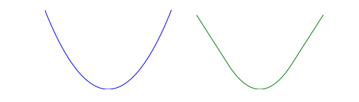
A more sophisticated variant is to replace the square function with the Huber function

\[\begin{split} \phi(u) = \left\{ \begin{array}{ll} u^2 & |u|\leq M\\ 2Mu - M^2 & |u|>M \end{array}\right. \end{split}\]

where \(M>0\) is the Huber threshold. The image below shows the square function on the left and the Huber function on the right.

Huber regression is the same as standard (least-squares) regression for small residuals, but allows (some) large residuals.

Example

In the following code we do a numerical example of Huber regression. We generate \(m=450\) measurements with \(n=300\) regressors. We randomly choose \(\beta^\mathrm{true}\) and \(x_i \sim \mathcal N(0,I)\). We set \(y_i = (\beta^\mathrm{true})^Tx_i + \epsilon_i\), where \(\epsilon_i \sim \mathcal N(0,1)\). Then with probability \(p\) we replace \(y_i\) with \(-y_i\).

The data has fraction \(p\) of (non-obvious) wrong measurements. The distribution of “good” and “bad” \(y_i\) are the same.

Our goal is to recover \(\beta^\mathrm{true} \in {\bf R}^n\) from the measurements \(y\in {\bf R}^m\). We compare three approaches: standard regression, Huber regression, and “prescient” regression, where we know which measurements had their sign flipped.

We generate \(50\) problem instances, with \(p\) varying from \(0\) to \(0.15\), and plot the relative error in reconstructing \(\beta^\mathrm{true}\) for the three approaches. Notice that in the range \(p \in [0,0.08]\), Huber regression matches prescient regression. Standard regression, by contrast, fails even for very small \(p\).

# Generate data for Huber regression.
import numpy as np

np.random.seed(1)
n = 300
SAMPLES = int(1.5 * n)
beta_true = 5 * np.random.normal(size=(n, 1))
X = np.random.randn(n, SAMPLES)
Y = np.zeros((SAMPLES, 1))
v = np.random.normal(size=(SAMPLES, 1))

# Generate data for different values of p.
# Solve the resulting problems.
# WARNING this script takes a few minutes to run.
import cvxpy as cp

TESTS = 50
lsq_data = np.zeros(TESTS)
huber_data = np.zeros(TESTS)
prescient_data = np.zeros(TESTS)
p_vals = np.linspace(0, 0.15, num=TESTS)
for idx, p in enumerate(p_vals):
    # Generate the sign changes.
    factor = 2 * np.random.binomial(1, 1 - p, size=(SAMPLES, 1)) - 1
    Y = factor * X.T.dot(beta_true) + v

    # Form and solve a standard regression problem.
    beta = cp.Variable((n, 1))
    fit = cp.norm(beta - beta_true) / cp.norm(beta_true)
    cost = cp.norm(X.T @ beta - Y)
    prob = cp.Problem(cp.Minimize(cost))
    prob.solve()
    lsq_data[idx] = fit.value

    # Form and solve a prescient regression problem,
    # i.e., where the sign changes are known.
    cost = cp.norm(cp.multiply(factor, X.T @ beta) - Y)
    cp.Problem(cp.Minimize(cost)).solve()
    prescient_data[idx] = fit.value

    # Form and solve the Huber regression problem.
    cost = cp.sum(cp.huber(X.T @ beta - Y, 1))
    cp.Problem(cp.Minimize(cost)).solve()
    huber_data[idx] = fit.value

# Plot the relative reconstruction error for
# least-squares, prescient, and Huber regression.
import matplotlib.pyplot as plt

%config InlineBackend.figure_format = 'svg'

plt.plot(p_vals, lsq_data, label="Least squares")
plt.plot(p_vals, huber_data, label="Huber")
plt.plot(p_vals, prescient_data, label="Prescient")
plt.ylabel(r"$\||\beta - \beta^{\mathrm{true}}\||_2/\||\beta^{\mathrm{true}}\||_2$")
plt.xlabel("p")
plt.legend(loc="upper left")
plt.show()

# Plot the relative reconstruction error for Huber and prescient regression,
# zooming in on smaller values of p.
indices = np.where(p_vals <= 0.08)

plt.plot(p_vals[indices], huber_data[indices], "g", label="Huber")
plt.plot(p_vals[indices], prescient_data[indices], "r", label="Prescient")
plt.ylabel(r"$\||\beta - \beta^{\mathrm{true}}\||_2/\||\beta^{\mathrm{true}}\||_2$")
plt.xlabel("p")
plt.xlim([0, 0.07])
plt.ylim([0, 0.05])
plt.legend(loc="upper left")
plt.show()