Hello World#
%matplotlib inline
import pandas as pd
import cvxportfolio as cp
Download the problem data with yfinance. We select five liquid stocks.
import yfinance
tickers = ["AMZN", "AAPL", "MSFT", "GOOGL", "TSLA"]
# start_date = "2012-01-01"
# end_date = "2016-12-31"
returns = pd.DataFrame(
    dict(
        [
            (
                ticker,
                yfinance.download(ticker)[ #, start_date=start_date, end_date=end_date)[
                    "Adj Close"
                ].pct_change(),
            )
            for ticker in tickers
        ]
    )
)
[*********************100%***********************] 1 of 1 completed
[*********************100%***********************] 1 of 1 completed
[*********************100%***********************] 1 of 1 completed
[*********************100%***********************] 1 of 1 completed
[*********************100%***********************] 1 of 1 completed
returns.describe()
| AMZN | AAPL | MSFT | GOOGL | TSLA | |
|---|---|---|---|---|---|
| count | 6523.000000 | 10675.000000 | 9349.000000 | 4697.000000 | 3222.000000 |
| mean | 0.001704 | 0.001100 | 0.001134 | 0.000983 | 0.002125 |
| std | 0.036077 | 0.028212 | 0.021314 | 0.019434 | 0.036126 |
| min | -0.247661 | -0.518692 | -0.301159 | -0.116341 | -0.210628 |
| 25% | -0.013295 | -0.013056 | -0.009217 | -0.007995 | -0.015596 |
| 50% | 0.000402 | 0.000000 | 0.000352 | 0.000745 | 0.001218 |
| 75% | 0.014799 | 0.014695 | 0.011355 | 0.010087 | 0.019381 |
| max | 0.344714 | 0.332280 | 0.195652 | 0.199915 | 0.243951 |
We get the return on cash from FRED.
import pandas_datareader

returns[["USDOLLAR"]] =  pandas_datareader.get_data_fred("DFF", start='2000-01-01') / (250 * 100)
returns = returns.fillna(method="ffill").dropna()

returns.tail()
| AMZN | AAPL | MSFT | GOOGL | TSLA | USDOLLAR | |
|---|---|---|---|---|---|---|
| Date | ||||||
| 2023-04-12 | -0.020917 | -0.004353 | 0.002334 | -0.006739 | -0.033460 | 0.000193 |
| 2023-04-13 | 0.046714 | 0.034104 | 0.022399 | 0.026663 | 0.029689 | 0.000193 |
| 2023-04-14 | 0.001074 | -0.002114 | -0.012766 | 0.013404 | -0.004841 | 0.000193 |
| 2023-04-17 | 0.002244 | 0.000121 | 0.009296 | -0.026637 | 0.011027 | 0.000193 |
| 2023-04-18 | -0.006619 | 0.004600 | -0.004778 | -0.008116 | -0.012992 | 0.000193 |
We compute rolling estimates of the first and second moments of the returns using a window of 1000 days. We shift them by one unit (so at every day we present the optimizer with only past data).
r_hat = returns.rolling(window=1000).mean().shift(1).dropna()
Sigma_hat = returns.shift(1).rolling(window=1000).cov().dropna()

r_hat
| AMZN | AAPL | MSFT | GOOGL | TSLA | USDOLLAR | |
|---|---|---|---|---|---|---|
| Date | ||||||
| 2014-06-20 | 0.001314 | 0.001108 | 0.000786 | 0.001036 | 0.002961 | 0.000005 |
| 2014-06-23 | 0.001300 | 0.001116 | 0.000803 | 0.001059 | 0.002971 | 0.000005 |
| 2014-06-24 | 0.001293 | 0.001127 | 0.000804 | 0.001085 | 0.003083 | 0.000005 |
| 2014-06-25 | 0.001300 | 0.001127 | 0.000794 | 0.001089 | 0.003189 | 0.000005 |
| 2014-06-26 | 0.001302 | 0.001121 | 0.000777 | 0.001113 | 0.003368 | 0.000005 |
| ... | ... | ... | ... | ... | ... | ... |
| 2023-04-12 | 0.000320 | 0.001412 | 0.001074 | 0.000738 | 0.003294 | 0.000048 |
| 2023-04-13 | 0.000280 | 0.001393 | 0.001063 | 0.000718 | 0.003256 | 0.000048 |
| 2023-04-14 | 0.000338 | 0.001429 | 0.001089 | 0.000753 | 0.003306 | 0.000049 |
| 2023-04-17 | 0.000339 | 0.001436 | 0.001043 | 0.000761 | 0.003343 | 0.000049 |
| 2023-04-18 | 0.000316 | 0.001441 | 0.001047 | 0.000726 | 0.003405 | 0.000049 |
2222 rows × 6 columns
Sigma_hat
| AMZN | AAPL | MSFT | GOOGL | TSLA | USDOLLAR | ||
|---|---|---|---|---|---|---|---|
| Date | |||||||
| 2014-06-20 | AMZN | 4.237160e-04 | 1.014461e-04 | 9.996433e-05 | 1.531471e-04 | 2.003648e-04 | 9.720131e-10 |
| AAPL | 1.014461e-04 | 2.841137e-04 | 7.152255e-05 | 1.037271e-04 | 1.220260e-04 | -6.378275e-10 | |
| MSFT | 9.996433e-05 | 7.152255e-05 | 1.983346e-04 | 8.818659e-05 | 1.074351e-04 | -7.018987e-10 | |
| GOOGL | 1.531471e-04 | 1.037271e-04 | 8.818659e-05 | 2.528908e-04 | 1.364906e-04 | 2.541239e-10 | |
| TSLA | 2.003648e-04 | 1.220260e-04 | 1.074351e-04 | 1.364906e-04 | 1.424632e-03 | -6.411383e-10 | |
| ... | ... | ... | ... | ... | ... | ... | ... |
| 2023-04-18 | AAPL | 3.212597e-04 | 4.669670e-04 | 3.427499e-04 | 3.168139e-04 | 4.707923e-04 | -1.459881e-08 |
| MSFT | 3.287896e-04 | 3.427499e-04 | 4.118900e-04 | 3.408980e-04 | 4.190421e-04 | 1.773549e-09 | |
| GOOGL | 3.220580e-04 | 3.168139e-04 | 3.408980e-04 | 4.396580e-04 | 3.835795e-04 | -2.223956e-08 | |
| TSLA | 4.559975e-04 | 4.707923e-04 | 4.190421e-04 | 3.835795e-04 | 1.848895e-03 | -1.065242e-07 | |
| USDOLLAR | -2.047893e-08 | -1.459881e-08 | 1.773549e-09 | -2.223956e-08 | -1.065242e-07 | 3.357492e-09 |
13332 rows × 6 columns
For the cash return instead we simply use the previous day’s return.
r_hat['USDOLLAR'] = returns['USDOLLAR'].shift(1)
Here we define the transaction cost and holding cost model (sections 2.3 and 2.4 of the paper). The data can be expressed as
a scalar (like we’re doing here), the same value for all assets and all time periods;
a Pandas Series indexed by the asset names, for asset-specific values;
a Pandas DataFrame indexed by timestamps with asset names as columns, for values that vary by asset and in time.
tcost_model = cp.TcostModel(half_spread=10e-4)
hcost_model = cp.HcostModel(borrow_costs=1e-4)
We define the single period optimization policy (section 4 of the paper).
risk_model = cp.FullCovariance(Sigma_hat)
gamma_risk, gamma_trade, gamma_hold = 1.0, 1.0, 1.0
leverage_limit = cp.LeverageLimit(3)

spo_policy = cp.SinglePeriodOpt(
    return_forecast=r_hat,
    costs=[
        gamma_risk * risk_model,
        gamma_trade * tcost_model,
        gamma_hold * hcost_model,
    ],
    constraints=[leverage_limit],
)
We run a backtest, which returns a result object. By calling its summary method we get some basic statistics.
market_sim = cp.MarketSimulator(
    returns, [tcost_model, hcost_model], cash_key="USDOLLAR"
)
init_portfolio = pd.Series(index=returns.columns, data=250000.0)
init_portfolio.USDOLLAR = 0
results = market_sim.run_multiple_backtest(
    init_portfolio,
    start_time="2020-01-01",
    end_time="2023-04-01",
    policies=[spo_policy,
             cp.Hold()
            ],
)
results[0].summary()
---------------------------------------------------------------------------
RemoteTraceback                           Traceback (most recent call last)
RemoteTraceback:
"""
Traceback (most recent call last):
  File "/opt/hostedtoolcache/Python/3.10.11/x64/lib/python3.10/site-packages/multiprocess/pool.py", line 125, in worker
    result = (True, func(*args, **kwds))
  File "/opt/hostedtoolcache/Python/3.10.11/x64/lib/python3.10/site-packages/multiprocess/pool.py", line 48, in mapstar
    return list(map(*args))
  File "/home/runner/work/cvxportfolio/cvxportfolio/cvxportfolio/simulator.py", line 272, in _run_backtest
    return self.run_backtest(
  File "/home/runner/work/cvxportfolio/cvxportfolio/cvxportfolio/simulator.py", line 231, in run_backtest
    u = policy.get_trades(h, t)
  File "/home/runner/work/cvxportfolio/cvxportfolio/cvxportfolio/policies.py", line 493, in get_trades
    constraints += constr.weight_expr(t, wplus, z, value)
  File "/home/runner/work/cvxportfolio/cvxportfolio/cvxportfolio/constraints.py", line 47, in weight_expr
    result = self.compile_to_cvxpy(wplus, z, v)
NameError: name 'wplus' is not defined
"""

The above exception was the direct cause of the following exception:

NameError                                 Traceback (most recent call last)
Cell In[10], line 6
      4 init_portfolio = pd.Series(index=returns.columns, data=250000.0)
      5 init_portfolio.USDOLLAR = 0
----> 6 results = market_sim.run_multiple_backtest(
      7     init_portfolio,
      8     start_time="2020-01-01",
      9     end_time="2023-04-01",
     10     policies=[spo_policy,
     11              cp.Hold()
     12             ],
     13 )
     14 results[0].summary()

File ~/work/cvxportfolio/cvxportfolio/cvxportfolio/simulator.py:279, in MarketSimulator.run_multiple_backtest(self, initial_portf, start_time, end_time, policies, loglevel, parallel)
    277 if parallel:
    278     workers = multiprocess.Pool(num_workers)
--> 279     results = workers.map(_run_backtest, policies)
    280     workers.close()
    281     return results

File /opt/hostedtoolcache/Python/3.10.11/x64/lib/python3.10/site-packages/multiprocess/pool.py:367, in Pool.map(self, func, iterable, chunksize)
    362 def map(self, func, iterable, chunksize=None):
    363     '''
    364     Apply `func` to each element in `iterable`, collecting the results
    365     in a list that is returned.
    366     '''
--> 367     return self._map_async(func, iterable, mapstar, chunksize).get()

File /opt/hostedtoolcache/Python/3.10.11/x64/lib/python3.10/site-packages/multiprocess/pool.py:774, in ApplyResult.get(self, timeout)
    772     return self._value
    773 else:
--> 774     raise self._value

NameError: name 'wplus' is not defined
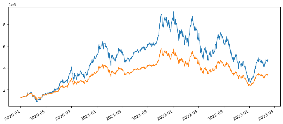
The total value of the portfolio in time.
results[1].summary()
Number of periods                               818
Initial timestamp               2020-01-02 00:00:00
Final timestamp                 2023-03-31 00:00:00
Portfolio return (%)                         41.343
Excess return (%)                            40.340
Excess risk (%)                              45.013
Sharpe ratio                                  0.897
Max. drawdown                                59.516
Turnover (%)                                  0.000
Average policy time (sec)                     0.000
Average simulator time (sec)                  0.001
results[0].v.plot(figsize=(12, 5))
results[1].v.plot(figsize=(12, 5))
<Axes: >
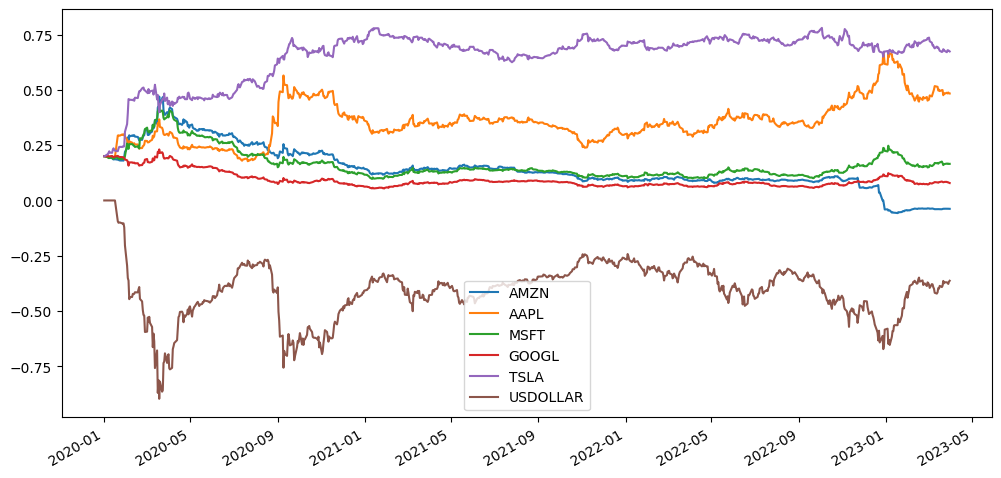
The weights vector of the portfolio in time.
results[0].w.plot(figsize=(12, 6))
<Axes: >